Atomic Vibration Frequency
To follow this tutorial, please download and unzip Example4/ from this link (154 MB).
Although the atomic vibration frequency (\(\nu^*\)) and the attempt frequency (\(\nu\)) are often used interchangeably, they are fundamentally different. The atomic vibration frequency is a result of all phonon modes within the system. In contrast, the attempt frequency is typically associated with a single phonon branch relevant to a specific hopping path. Users should carefully consider which of these values is appropriate for their analysis.
In VacHopPy, the atomic vibration frequency is primarily used to determine the optimal t_interval, which is calculated as \(1/\nu^*\).
How to Calculate the Atomic Vibration Frequency
VacHopPy provides the vibration command to calculate the atomic vibration frequency.
vachoppy vibration [PATH_TRAJ] [PATH_STRUCTURE] [SYMBOL]
Command Arguments
This command takes the following primary arguments:
PATH_TRAJPath to a single HDF5 trajectory file.
PATH_STRUCTUREPath to a structure file of the perfect, vacancy-free material. While this example uses VASP POSCAR, any format supported by the Atomic Simulation Environment (ASE) is compatible.
SYMBOLThe chemical symbol of the diffusing species (e.g., O for oxygen).
Key Optional Flags
--sampling_sizeBy default,
VacHopPyanalyzes only the first 5000 frames of the HDF5 file, as the vibration frequency typically converges quickly within a few thousand frames. If the file contains fewer than 5000 frames, the entire file is used. You can change this behavior by setting a different number with this flag.--no-filterHigh-frequency regions in the analysis can sometimes contain non-physical artifacts.
VacHopPyautomatically filters these high frequencies using an Interquartile Range (IQR) method. To disable this feature, use the--no-filterflag.
Running the Analysis
Navigate into the Example4/ directory you downloaded. In this directory, you will find two files:
cd path/to/Example4/
ls
# >> POSCAR_TiO2  TRAJ_O_01.h5
TRAJ_O_01.h5: ThePATH_TRAJfile, containing an MD simulation of a rutile TiO₂ supercell with one oxygen vacancy at 2100 K.POSCAR_TiO2: ThePATH_STRUCTUREfile, containing the structure of the perfect, vacancy-free rutile TiO₂ supercell.
Execute the following command to run the analysis:
vachoppy vibration TRAJ_O_01.h5 POSCAR_TiO2 O
Understanding the Output
The command prints the calculation results to the terminal and generates two image files (displacement.png and frequency.png) in a new imgs/ directory.
Terminal Output
The terminal first shows progress bars for the analysis, followed by a summary of the results. By default, the high-frequency filter is enabled, and its results are displayed first.
[STEP1] Atomic Vibration Analysis (Using initial 5000 frames):
Compute Displacement: 100%|##############################| 47/47 [00:00<00:00, 49.15it/s]
Capture Vibrations : 100%|##############################| 5000/5000 [00:03<00:00, 1573.98it/s]
Compute Frequenciy : 100%|##############################| 47/47 [00:00<00:00, 3609.69it/s]
====================================================
High-Frequency Filtering Results (IQR)
====================================================
- Cutoff Frequency : 32.14 THz
- Removed Outlier Frequencies : 74 (out of 7521)
====================================================
Vibrational Analysis Results Summary
====================================================
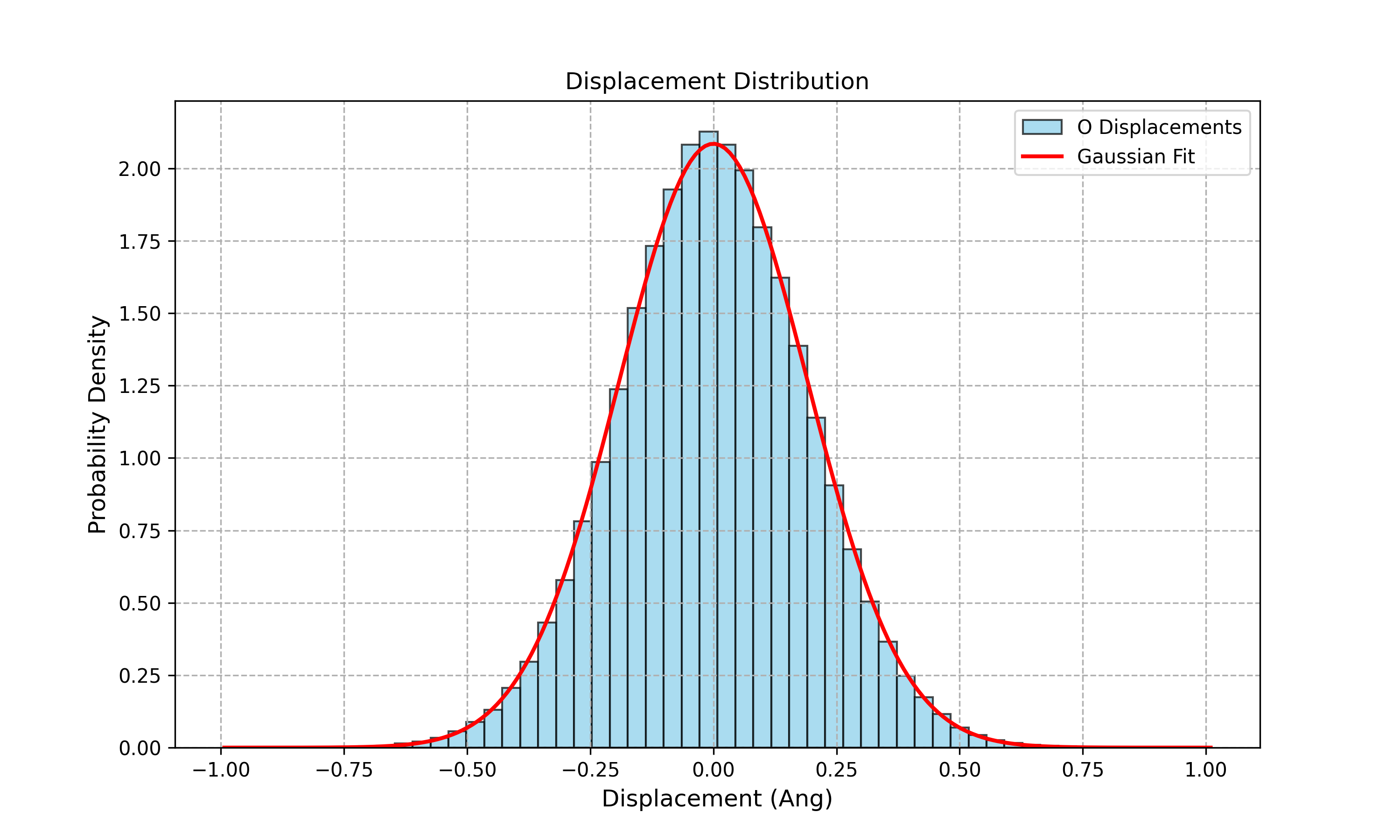
- Mean Vibrational Amplitude (σ) : 0.191 Ang
- Determined Site Radius (2 x σ) : 0.383 Ang
- Total Vibrational Frequencies : 7447 found
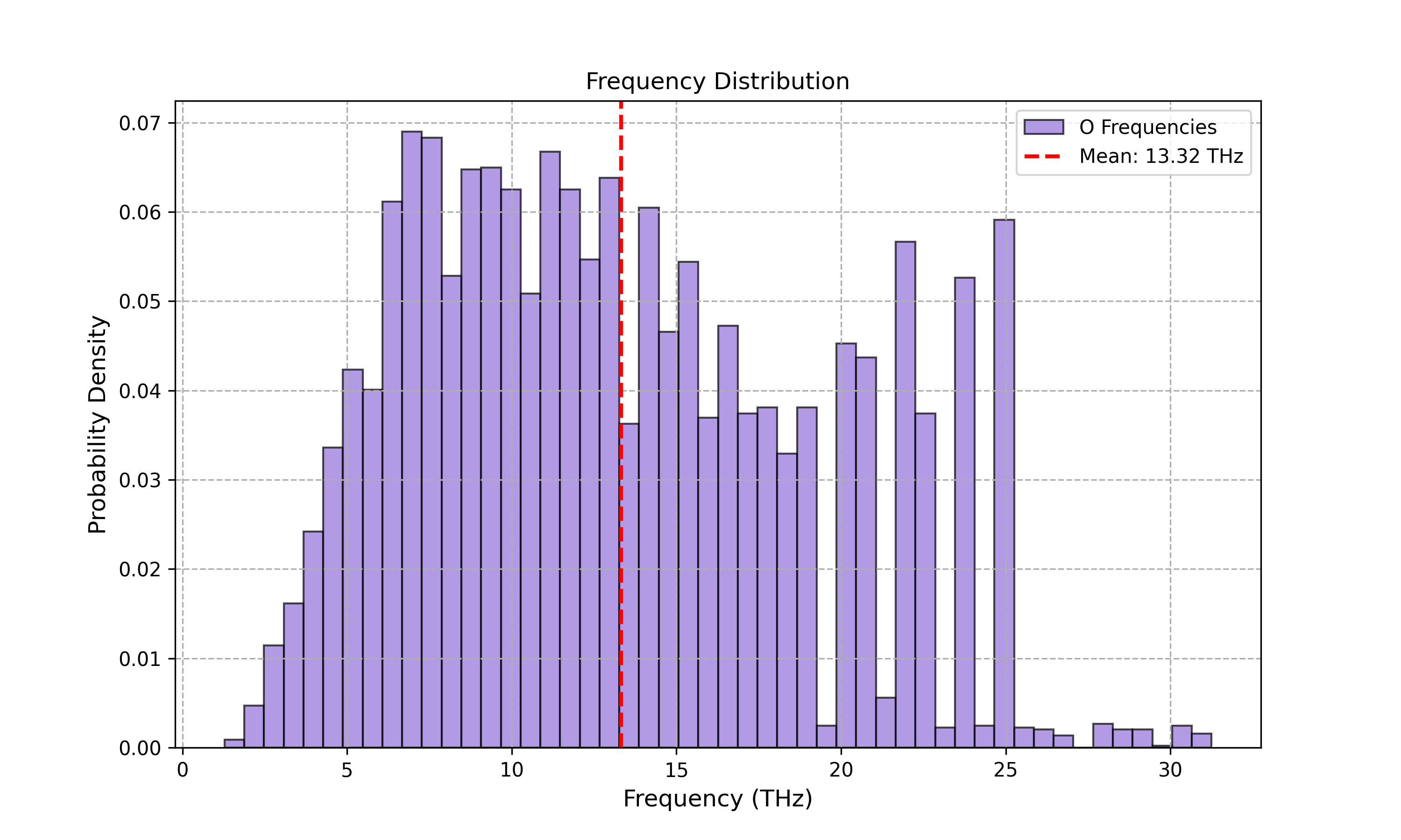
- Mean Vibrational Frequency : 13.324 THz
====================================================
Images are saved in 'imgs'.
Execution Time: 10.514 seconds
Peak RAM Usage: 0.022 GB
Generated Files
VacHopPy generates two plots to help visualize the results, which are saved in the imgs/ directory.
Displacement Distribution
This plot shows the distribution of atomic displacements from their equilibrium lattice sites.
Frequency Distribution
This plot shows the distribution of the calculated atomic vibration frequencies, which are obtained via a Fourier transform of the displacements.