Mean Square Displacement
To follow this tutorial, please download and unzip Example3/ from this link (26 GB).
Note
This is the same example set used in the Hopping Parameter Extraction section. If you have already completed that tutorial, you do not need to download the files again.
How to Calculate MSD-based Diffusivity
VacHopPy provides the msd command for performing Mean Squared Displacement (MSD) analysis. Unlike the analyze command, which calculates vacancy diffusivity (\(D\)) based on site occupations, the msd command tracks the movement of the atoms themselves to calculate the atomic diffusivity (\(D_{atom}\)).
where \(x_{vac}\) is the mole fraction of vacancies in the system.
The basic syntax for the msd command is:
vachoppy msd [PATH_TRAJ] [SYMBOL]
Command Arguments
PATH_TRAJPath to either a single HDF5 trajectory file or a root directory containing multiple files. If data from multiple temperatures is provided, an Arrhenius analysis is automatically performed.
SYMBOLThe chemical symbol of the diffusing species (e.g., O for oxygen).
Key Optional Flags
--skipInitial time in picoseconds (ps) to exclude from the analysis, useful for ignoring initial equilibration steps. (Default: 0.0)
--startStart time in picoseconds (ps) for the linear fitting range of the MSD plot. This is used to exclude the initial ballistic transport regime. (Default: 1.0)
--endEnd time in picoseconds (ps) for the linear fitting range. (Default: None)
--segment_lengthSplits a long trajectory into several shorter segments of a given length (ps) and analyzes them as parallel simulations. For example,
--segment_length 10on a 30 ps trajectory treats the data as three independent 10 ps simulations. You can provide a single value for all temperatures or a list of values for each temperature.--n_jobsNumber of CPU cores for parallel processing. (Default: -1, uses all available cores)
--depthMaximum directory depth to search for trajectory files. (Default: 2)
Running the Analysis
Navigate into the Example3/ directory you downloaded. For this tutorial, we will only use the TRAJ_TiO2/ directory.
cd path/to/Example3/
ls
# >> TRAJ_TiO2/  POSCAR_TiO2  neb_TiO2.csv
The TRAJ_TiO2/ directory contains the HDF5 files from MD simulations performed at five temperatures. Inside, it has subdirectories for each temperature (TRAJ_1700K/ through TRAJ_2100K/). Each of these subdirectories contains 20 individual HDF5 files (e.g., TRAJ_O_01.h5 to TRAJ_O_20.h5) of the same NVT ensemble.
Usage Scenarios for the msd Command
The msd command is flexible and can be used in several ways depending on your analysis needs:
To analyze a single HDF5 file:
Calculates MSD and \(D_{atom}\) for one run
# Analyzes a single trajectory file from the 2100 K simulation
vachoppy analyze TRAJ_TiO2/TRAJ_2100K/TRAJ_O_01.h5 O
To analyze a single-temperature ensemble:
Calculates average MSD and \(D_{atom}\) for that temperature
# Analyzes all 20 trajectory files from the 2100 K simulation
vachoppy analyze TRAJ_TiO2/TRAJ_2100K/ O
To analyze a multi-temperature ensemble:
Calculates \(D_{atom}\) for each temperature and performs an Arrhenius fit
# Analyzes all 100 trajectory files from 1700 K to 2100 K
vachoppy msd TRAJ_TiO2/ O
Advanced Usage with --segment_length
You can use the --segment_length flag to split long simulations into shorter segments for statistical analysis.
To apply the same segment length to all temperatures:
# Each simulation at every temperature is analyzed in 50 ps segments
vachoppy msd TRAJ_TiO2/ O --segment_length 50
To apply different segment lengths to each temperature:
# Applies 50 ps for the first three temps (1700K, 1800K, 1900K)
# and 100 ps for the last two (2000K, 2100K)
vachoppy msd TRAJ_TiO2/ O --segment_length 50 50 50 100 100
For this tutorial, we will run the analysis with the default settings. Note that tuning parameters like --skip, --start, --end, and --segment_length can significantly improve the quality of your results by ensuring the analysis is performed on the linear, diffusive regime of the MSD plot.
Execute the following command:
vachoppy msd TRAJ_TiO2/ P O --neb neb_TiO2.csv
Understanding the Output
The command prints a detailed summary to the terminal, generates msd.png and D_atom.png image files in the imgs/ directory, and saves the raw calculated data to einstein.json.
Terminal Output
[STEP1] MSD Calculation Based on Einstein Relation:
Compute MSD: 100%|##############################| 100/100 [00:03<00:00, 26.17it/s]
Execution Time: 5.637 seconds
Peak RAM Usage: 0.212 GB
[STEP2] Summary of MSD Analysis:
==================================================
MSD Ensemble Analysis Summary
==================================================
Temp (K) Avg. Diffusivity (m^2/s)
---------- --------------------------
1700 8.616e-12
1800 1.307e-11
1900 1.686e-11
2000 2.251e-11
2100 2.948e-11
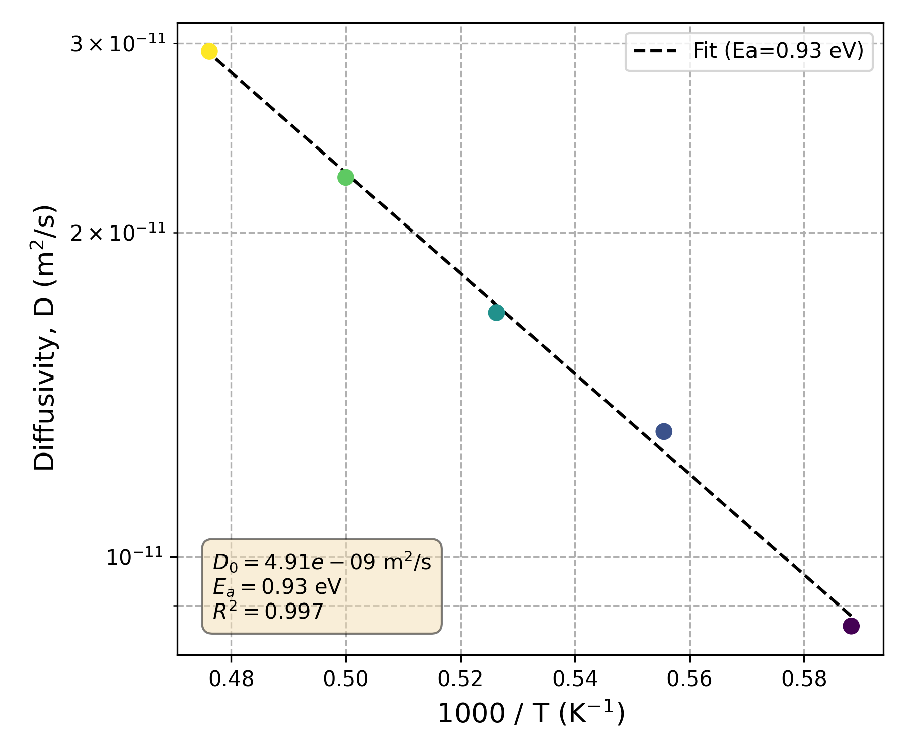
-- Arrhenius Fit Results --
- Activation Energy (Ea) : 0.927 eV
- Pre-factor (D0) : 4.914e-09 m^2/s
- R-squared : 0.9970
==================================================
Results are saved in 'einstein.json'.
Images are saved in imgs.
Execution Time: 13.773 seconds
Peak RAM Usage: 0.000 GB
Generated Files
VacHopPy generates two plots to help visualize the results, which are saved in the imgs/ directory.
Image Files for Visualization
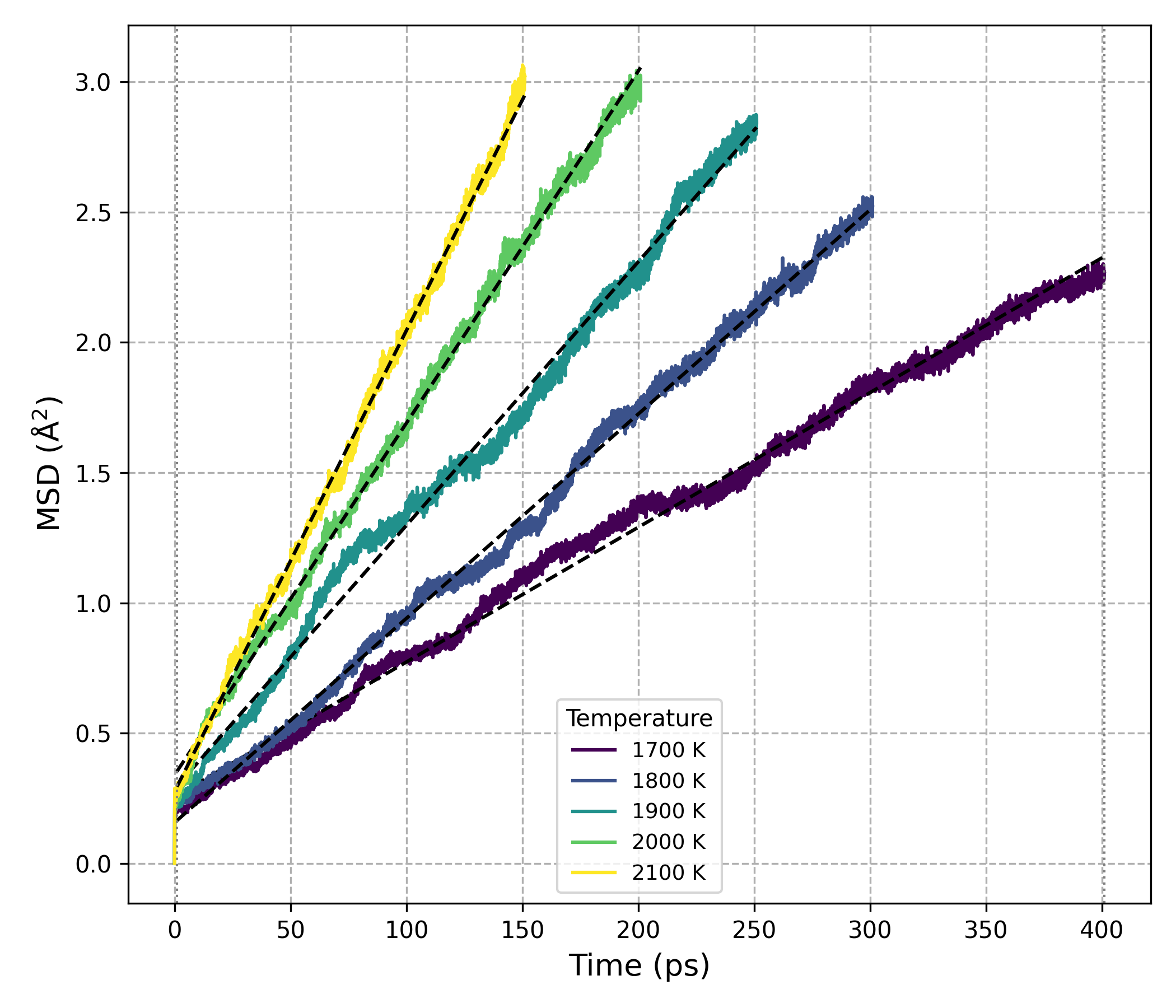
MSD vs. Time
This plot shows the MSD as a function of time for each temperature.
Arrhenius Plot for Atomic Diffusivity
This plot shows the temperature dependence of the atomic diffusivity and the corresponding Arrhenius fit.
The raw calculated data is saved in einstein.json. This file contains the temperature-dependent results and fitted parameters, along with a description key explaining each value.
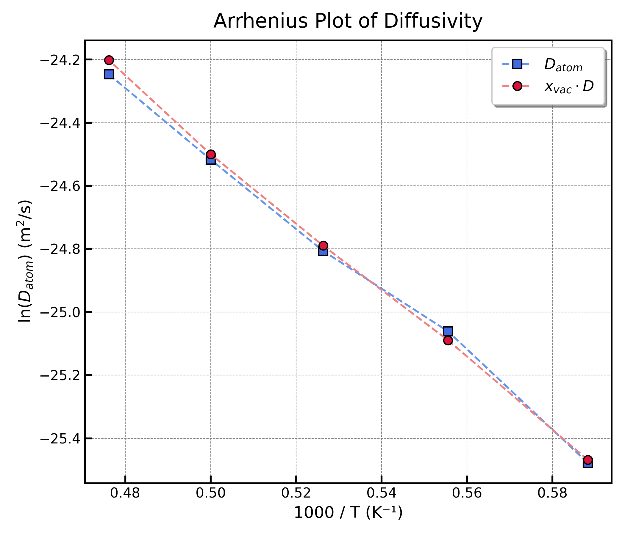
Comparison: Site-Occupation vs. MSD Diffusivity
Ideally, the atomic diffusivity (\(D_{atom}\)) from the msd command should match the vacancy diffusivity (\(D\)) from the analyze command according to the equation (1) discussed earlier.
However, results may differ slightly. The MSD-based calculation includes all thermal fluctuations and can be influenced by other transport mechanisms beyond pure vacancy-mediated diffusion (e.g., collective atomic movements).
The plot below compares the final calculated values of \(D_{atom}\) and \(x_{vac} \cdot D\) for our example system, showing good agreement.