Hopping Parameter Extraction

To follow this tutorial, please download and unzip Example3/ from this link (26 GB).

---

How to Extract Hopping Parameters

The core feature of VacHopPy—calculating effective hopping parameters—is automated by the analyze command. The basic syntax is as follows:

vachoppy analyze [PATH_TRAJ] [PATH_STRUCTURE] [SYMBOL] --neb [NEB_CSV]

Command Arguments

This command takes the following primary arguments:

• PATH_TRAJ

  Path to either a single HDF5 trajectory file or a root directory containing multiple HDF5 files. If files from multiple temperatures are provided, an Arrhenius-type analysis is automatically performed.

• PATH_STRUCTURE

  Path to a structure file of the perfect, vacancy-free material. While this example uses VASP POSCAR, any format supported by the Atomic Simulation Environment (ASE) is compatible. VacHopPy uses this file to determine lattice sites and potential hopping paths.

• SYMBOL

  The chemical symbol of the diffusing species (e.g., O for oxygen).

• --neb [NEB_CSV] (Optional)

  Path to a CSV file containing the activation energy barrier for each hopping path, as pre-calculated from a method like nudged elastic band (NEB).

The NEB_CSV File

This optional CSV file provides essential energy information for calculating certain parameters like the attempt frequency (\(\nu\)) and coordination number (\(z\)). The format is a simple two-column list of path names and their corresponding energy barriers in eV.

Example neb_TiO2.csv:

A1,0.8698
A2,1.058
A3,1.766

The required path names (e.g., A1, A2) can be identified using the Site class.

from vachoppy.core import Site

site = Site([PATH_STRUCTURE], [SYMBOL]) 
site.summary()

Running the summary() method provides the necessary structural information about crystal sites and potential hopping paths.

Example output:

==============================================================================================================
                                             Site Analysis Summary
==============================================================================================================
  - Structure File       : POSCAR_TiO2
  - Diffusing Symbol     : O
  - Inequivalent Sites   : 1 found
  - Inequivalent Paths   : 3 found (with Rmax = 3.25 Å)

-- Hopping Path Information --

Name    Init Site    Final Site    a (Å)    z    Initial Coord (Frac)      Final Coord (Frac)
------  -----------  ------------  -------  ---  ------------------------  -------------------------
A1      site1        site1         2.5626   1    [0.0975, 0.4025, 0.1667]  [-0.0975, 0.5975, 0.1667]
A2      site1        site1         2.8031   8    [0.0975, 0.4025, 0.1667]  [0.3475, 0.3475, 0.3333]
A3      site1        site1         2.967    2    [0.0975, 0.4025, 0.1667]  [0.0975, 0.4025, -0.1667]
==============================================================================================================

List of Extractable Parameters

The specific effective hopping parameters that VacHopPy can calculate depend entirely on the data you provide. There are two factors:

• Number of Temperatures

  Do your HDF5 files represent a single temperature or a range of temperatures?

• NEB_CSV

  Have you provided a CSV file with pre-calculated hopping barriers?

The following table summarizes what can be calculated under different conditions. (O = Calculable, X = Not Calculable).

Parameter	Symbol	Single T	Multiple T	NEB_CSV Required?
Diffusivity	\(D\)	O	O	No
Residence Time	\(\tau\)	O	O	No
Correlation Factor	\(f\)	O	O	No
Hopping Barrier	\(E_a\)	X	O	No
Hopping Distance	\(a\)	O	O	No
Coordination Number	\(z\)	X	O	Yes
Attempt Frequency	\(\nu\)	O	O	Yes

---

Running the Analysis

Navigate into the Example3/ directory you downloaded. In this directory, you will find one subdirectory and two files:

cd path/to/Example3/
ls
# >> TRAJ_TiO2/  POSCAR_TiO2  neb_TiO2.csv

• TRAJ_TiO2/

  This directory contains the HDF5 files from MD simulations performed at multiple temperatures. Inside, it has subdirectories for each temperature (TRAJ_1700K/ through TRAJ_2100K/). Each of these subdirectories contains 20 individual HDF5 files (e.g., TRAJ_O_01.h5 to TRAJ_O_20.h5) of the same NVT ensemble.

• POSCAR_TiO2

  This is the structure file corresponding to the PATH_STRUCTURE argument. It contains the perfect, vacancy-free rutile TiO₂ supercell.

• neb_TiO2.csv This is the NEB_CSV file, which contains the pre-calculated hopping barrier information for the vacancy hopping paths identified from POSCAR_TiO2.

Usage Scenarios for the analyze Command

The analyze command is flexible and can be used in several ways depending on your analysis needs:

• To analyze a single HDF5 file:

# Analyzes a single trajectory file from the 2100 K simulation
vachoppy analyze TRAJ_TiO2/TRAJ_2100K/TRAJ_O_01.h5 POSCAR_TiO2 O --neb neb_TiO2.csv

• To analyze multiple HDF5 files from a single-temperature ensemble:

# Analyzes all 20 trajectory files from the 2100 K simulation
vachoppy analyze TRAJ_TiO2/TRAJ_2100K/ POSCAR_TiO2 O --neb neb_TiO2.csv

• To analyze multiple HDF5 files across a range of temperatures:

# Analyzes all 100 trajectory files from 1700 K to 2100 K
vachoppy analyze TRAJ_TiO2/ POSCAR_TiO2 O --neb neb_TiO2.csv

Key Optional Flags

• The --neb [NEB_CSV] flag can be omitted if you do not need to calculate parameters that depend on NEB data (like \(\nu\) and \(z\)).

• When PATH_TRAJ is a directory, VacHopPy automatically searches for HDF5 files up to two levels deep. You can adjust this search range using the --depth flag (default is 2).

• VacHopPy processes large datasets efficiently using streaming and parallel processing. You can control the number of CPU cores used with the --n_jobs flag. The default is -1, which uses all available cores.

Running the Full Tutorial Analysis

For this tutorial, we will demonstrate the full capabilities of VacHopPy by analyzing all 100 HDF5 files from 1700-2100 K, including the NEB_CSV file.

Execute the following command:

vachoppy analyze TRAJ_TiO2/ POSCAR_TiO2 O --neb neb_TiO2.csv

---

Understanding the Output

The command prints a detailed summary in the terminal and generates two types of files: several image files in a new imgs/ directory and a comprehensive parameters.json file.

Terminal Output

The command prints a multi-step summary direct to the terminal. Let’s break down each step.

• Step 1: Automatic t_interval Estimation

  The analysis begins by estimating the optimal time interval for analysis (t_interval) from a representative file for each temperature.

[STEP1] Automatic t_interval Estimation:
============================================================
               Automatic t_interval Estimation
============================================================
  [1700.0 K] Estimating from TRAJ_1700K/TRAJ_O_01.h5
             -> t_interval : 0.075 ps
  [1800.0 K] Estimating from TRAJ_1800K/TRAJ_O_01.h5
             -> t_interval : 0.075 ps
  [1900.0 K] Estimating from TRAJ_1900K/TRAJ_O_01.h5
             -> t_interval : 0.075 ps
  [2000.0 K] Estimating from TRAJ_2000K/TRAJ_O_01.h5
             -> t_interval : 0.075 ps
  [2100.0 K] Estimating from TRAJ_2100K/TRAJ_O_01.h5
             -> t_interval : 0.075 ps
============================================================
    Adjusting t_interval to the nearest multiple of dt
============================================================
    - dt                  : 0.0020 ps
    - Original t_interval : 0.0750 ps
    - Adjusted t_interval : 0.0740 ps (37 frames)
============================================================

• Step 2: Trajectory Analysis Progress

  Next, VacHopPy analyzes all 100 trajectory files in parallel, showing a progress bar.

[STEP2] Vacancy Trajectory Identification:
Analyze Trajectory: 100%|##############################| 100/100 [00:09<00:00, 10.70it/s]

• Step 3: Summary on Effective Hopping Parameters

  Once the analysis is complete, a summary of the calculated effective hopping parameters is displayed. This includes both the temperature-dependent data and the final parameters from the Arrhenius fits.

[STEP3] Hopping Parameter Calculation:
============================================================
Summary for Trajectory dataset
  - Path to TRAJ bundle : TRAJ_TiO2 (depth=2)
  - Lattice structure   : POSCAR_TiO2
  - t_interval          : 0.074 ps (37 frames)
  - Temperatures (K)    : [1700.0, 1800.0, 1900.0, 2000.0, 2100.0]
  - Num. of TRAJ files  : [20, 20, 20, 20, 20]
============================================================

================ Temperature-Dependent Data ================
Temp (K)    D (m2/s)    D_rand (m2/s)    f       tau (ps)    a (Ang)
----------  ----------  ---------------  ------  ----------  ---------
1700        4.176e-10   6.413e-10        0.6511  19.092      2.7104
1800        6.097e-10   9.179e-10        0.6642  13.3759     2.7142
1900        8.228e-10   1.249e-09        0.6589  9.938       2.7287
2000        1.099e-09   1.663e-09        0.661   7.4301      2.7227
2100        1.48e-09    2.262e-09        0.6543  5.4597      2.7224
============================================================

================= Final Fitted Parameters ==================
Diffusivity (D):
  - Ea          : 0.961 eV
  - D0          : 2.944e-07 m^2/s
  - R-squared   : 0.9991
Random Walk Diffusivity (D_rand):
  - Ea          : 0.958 eV
  - D0          : 4.413e-07 m^2/s
  - R-squared   : 0.9988
Correlation Factor (f):
  - Ea          : 0.002 eV
  - f0          : 0.667
  - R-squared   : 0.0218
Residence Time (tau):
  - Ea (fixed)  : 0.958 eV
  - tau0        : 2.777e-02 ps
  - R-squared   : 0.9987
============================================================

• Step 4: Attempt Frequency Summary

  Finally, if NEB_CSV file was provided, the results of the attempt frequency analysis are shown.

[STEP4] Attempt Frequency Calculation:
============================================================
            Attempt Frequency Analysis Summary
============================================================

-- Temperature-Dependent Effective Parameters --

Temp (K)    nu (THz)    z
----------  ----------  ------
1700.0      6.1675      5.8920
1800.0      6.0200      5.9904
1900.0      5.7611      6.0862
2000.0      5.6642      6.1788
2100.0      5.8308      6.2682
--------    --------    -
Mean        5.8887      6.0831

-- Path-Wise Parameters (per Temperature) --

Temperature: 1700.0 K
Path Name    Hop Count    nu_path (THz)
-----------  -----------  ---------------
A1           167          7.8923
A2           252          5.3794
A3           1            10.7228
----------------------------------------
Temperature: 1800.0 K
Path Name    Hop Count    nu_path (THz)
-----------  -----------  ---------------
A1           171          7.7409
A2           279          5.3119
A3           0            0
----------------------------------------
Temperature: 1900.0 K
Path Name    Hop Count    nu_path (THz)
-----------  -----------  ---------------
A1           161          6.5072
A2           344          5.4858
A3           0            0
----------------------------------------
Temperature: 2000.0 K
Path Name    Hop Count    nu_path (THz)
-----------  -----------  ---------------
A1           187          7.2352
A2           353          5.0879
A3           1            3.5067
----------------------------------------
Temperature: 2100.0 K
Path Name    Hop Count    nu_path (THz)
-----------  -----------  ---------------
A1           191          7.7369
A2           362          5.1858
A3           0            0
----------------------------------------
============================================================
NOTE: nu_paths can be unreliable for paths with low hop counts,
      as they are sensitive to statistical noise.
============================================================

Note

The automatic t_interval estimation (Step 1) is skipped if you manually provide a value with the --t_interval flag. The attempt frequency calculation (Step 4) is only performed if an NEB_CSV file is provided via the --neb flag.

Generated Files

VacHopPy generates several output files to help you understand and use the calculated parameters.

Image Files for Visualization

A series of plots are saved in the imgs/ directory to visualize the results. Below are a few key examples:

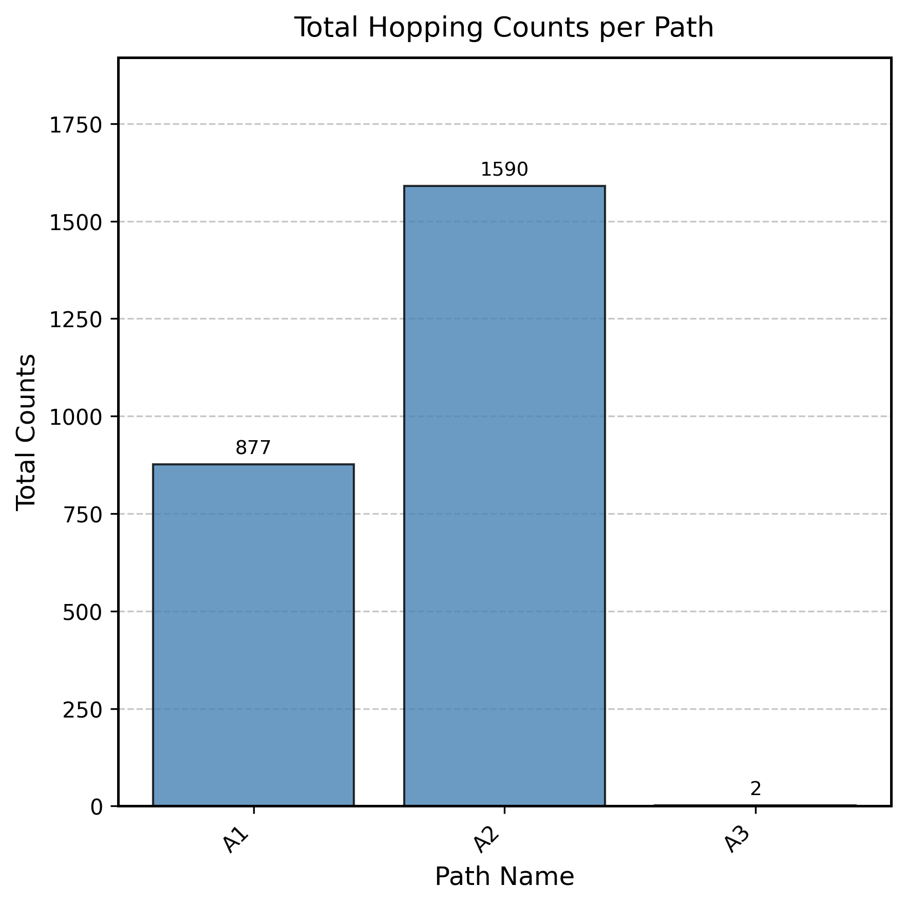
• Total Hopping Counts per Path

  This plot shows how frequently each type of hopping path was observed across all simulations.

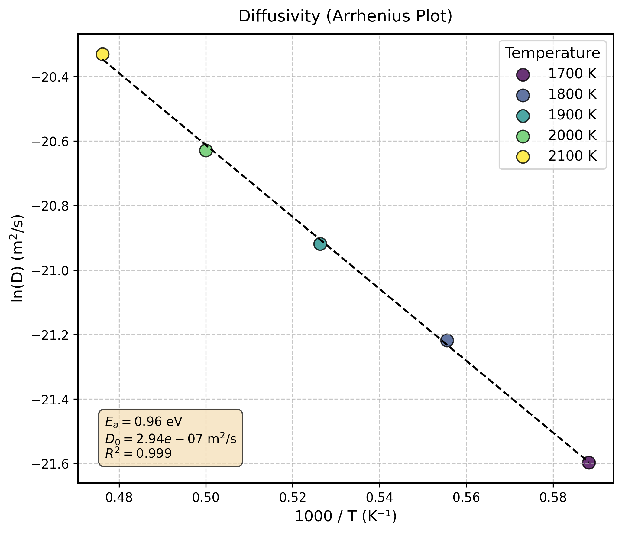
• Arrhenius plot for diffusivity

  This plot shows the temperature dependence of the vacancy diffusivity and the corresponding Arrhenius fit.

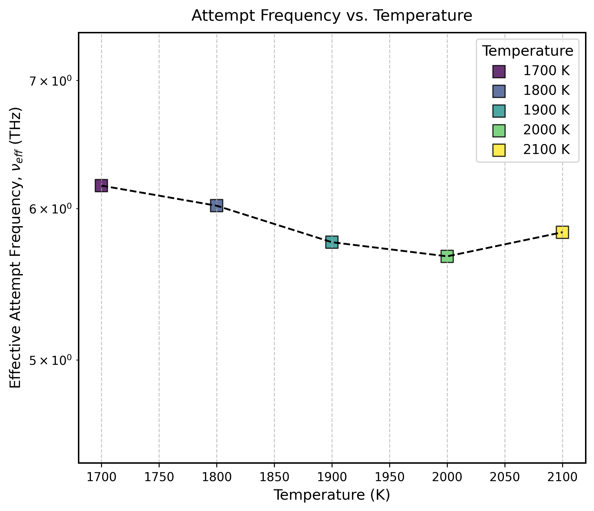
• Attempt Frequency vs Temperature

  This plot shows how the effective attempt frequency changes with temperature.

Other generated images (D_rand.png, f.png, tau.png, a.png, z.png) can also be found in the imgs/ directory.

The parameters.json File

This file contains all the raw calculated data in a machine-readable format. It also includes a helpful description key that provides a brief explanation for each parameter.

You can easily inspect the contents of this file with a simple Python script:

import json

with open('parameters.json', 'r') as f:
    params = json.load(f)

data = params['description']
max_key_length = max(len(k) for k in data.keys())

for k, v in data.items():
    print(f"{k:<{max_key_length}} : {v}")

Example output:

D          : Diffusivity (m2/s): (n_temperatures,)
D0         : Pre-exponential factor for diffusivity (m2/s)
Ea_D       : Activation barrier for diffusivity (eV)
D_rand     : Random walk diffusivity (m2/s): (n_temperatures,)
D_rand0    : Pre-exponential factor for random walk diffusivity (m2/s)
Ea_D_rand  : Activation barrier for random walk diffusivity (eV)
f          : Correlation factor: (n_temperatures,)
f0         : Pre-exponential factor for correlation factor
Ea_f       : Activation barrier for correlation factor (eV)
tau        : Residence time (ps): (n_temperatures,)
tau0       : Pre-exponential factor for residence time (ps)
Ea_tau     : Activation barrier for residence time (eV)
a          : Effective hopping distance (Ang) (n_temperatures,)
a_path     : Path-wise hopping distance (Ang): (n_paths,)
nu         : Effective attempt frequency (THz): (n_temperatures,)
nu_path    : Path-wise attempt frequency (THz): (n_temperatures, n_paths)
Ea_path    : Path-wise hopping barrier (eV): (n_paths)
z          : Effective number of the equivalent paths: (n_temperatures,)
z_path     : Number of the equivalent paths of each path: (n_paths,)
z_mean     : Mean number of the equivalent paths per path type: (n_temperatures,)
m_mean     : Mean number of path types: (n_temperatures,)
P_site     : Site occupation probability: (n_temperatures, n_sites)
P_esc      : Escape probability: (n_temperature, n_paths)
times_site : Total residence times at each site (ps): (n_temperature, n_sites)
counts_hop : Counts of hops at each temperature: (n_temperature, n_paths)

Note

A Note on Activation Barriers

In this context, it is crucial to distinguish between the hopping barrier and the diffusion barrier.

• The hopping barrier, represented by Ea_D_rand, is the activation energy for a single, random hop.

• The diffusion barrier, represented by Ea_D, is the total activation energy for the macroscopic diffusion process. It encompasses both the hopping barrier and the energetic contributions from jump correlations.

This subtle distinction is important. For instance, the activation energy that governs physical quantities like the residence time (\(\tau\)) or the hopping rate (\(\Gamma\)) corresponds to the hopping barrier (Ea_D_rand), not the overall diffusion barrier.

---

Advanced Features

Assessing Data Reliability

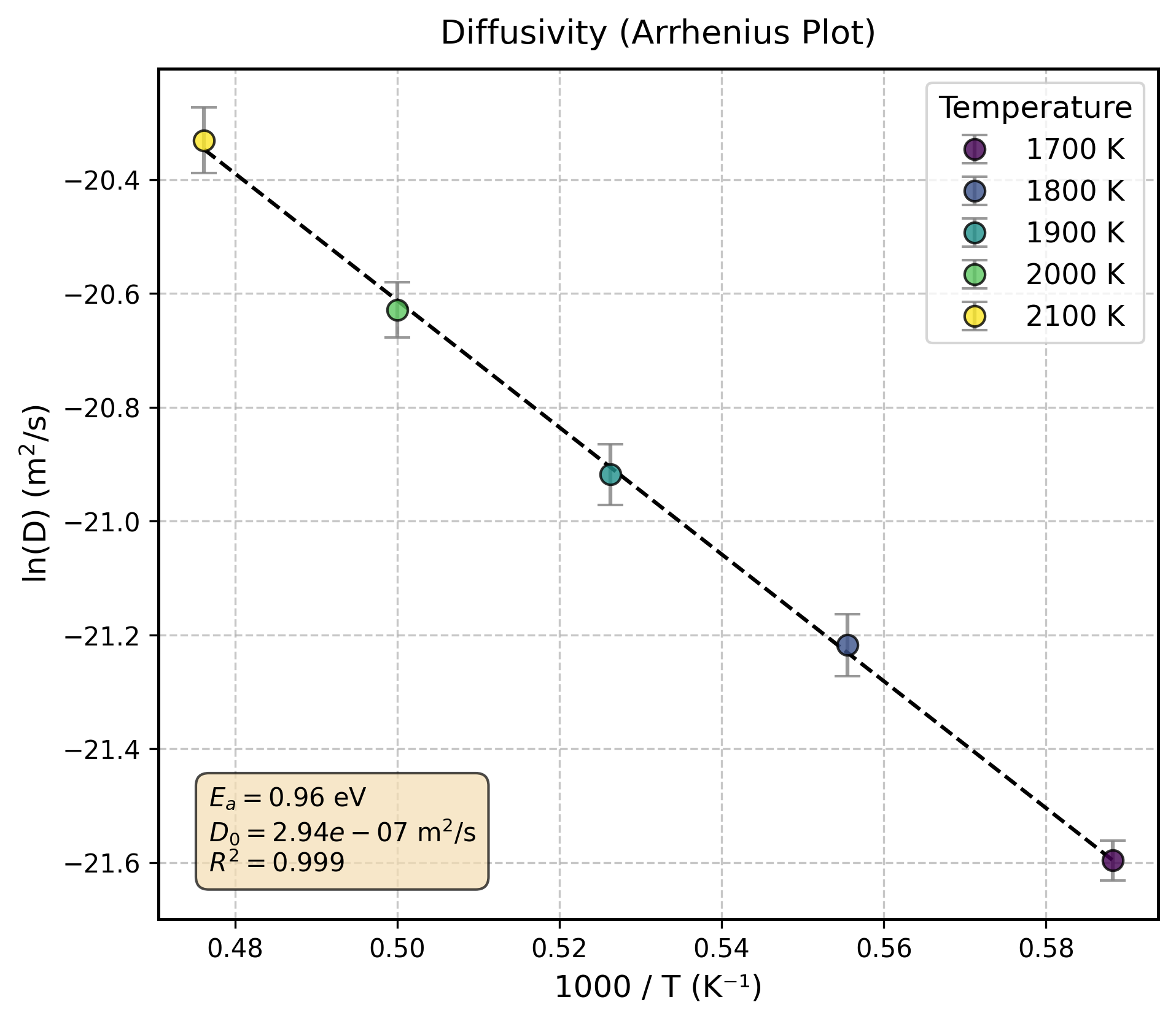
Using the --error_bar flag will display error bars on the plots for \(D\), \(D_{rand}\), \(f\), \(\tau\). The error bars represent the standard error of the mean (SEM), which allows for an assessment of the data’s reliability. It is calculated as follows:

\[ SEM = {\sigma}/{\sqrt{n}} \]

Here, \(\sigma\) represents the standard deviation of the physical quantity at each temperature, and \(n\) is the number of data points (i.e., the number of HDF5 files used for that temperature).

Below is an example of the output plot:

---

Decomposing Vacancy Diffusivity

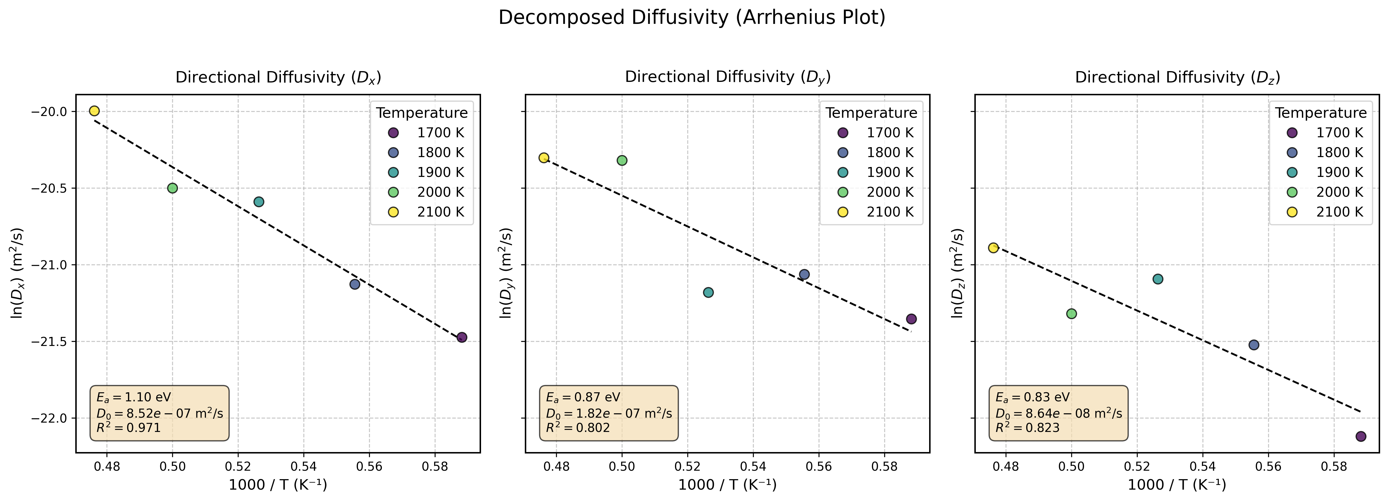
The --xyz flag enables the decomposition and analysis of vacancy diffusivity into its x, y, and z components. This analysis can be particularly effective when dealing with anisotropic systems.

Example terminal output:

[STEP5] Decomposing Diffusivity into xyz-Components:
=========== Temperature-Dependent Decomposed Diffusivity ===========
T (K)    Dx (m2/s)    Dy (m2/s)    Dz (m2/s)
-------  -----------  -----------  -----------
1700     4.729e-10    5.324e-10    2.475e-10
1800     6.673e-10    7.123e-10    4.496e-10
1900     1.144e-09    6.331e-10    6.915e-10
2000     1.25e-09     1.497e-09    5.507e-10
2100     2.069e-09    1.525e-09    8.47e-10
====================================================================

=================== Decomposed Diffusivity Fits ====================
Directional Diffusivity (Dx):
  - Ea        : 1.101 eV
  - D0        : 8.523e-07 m^2/s
  - R-squared : 0.9710
Directional Diffusivity (Dy):
  - Ea        : 0.867 eV
  - D0        : 1.818e-07 m^2/s
  - R-squared : 0.8022
Directional Diffusivity (Dz):
  - Ea        : 0.834 eV
  - D0        : 8.645e-08 m^2/s
  - R-squared : 0.8231
====================================================================

This flag also generates additional plots for the component-wise Mean Squared Displacement (MSD) and component-wise Arrhenius fits.

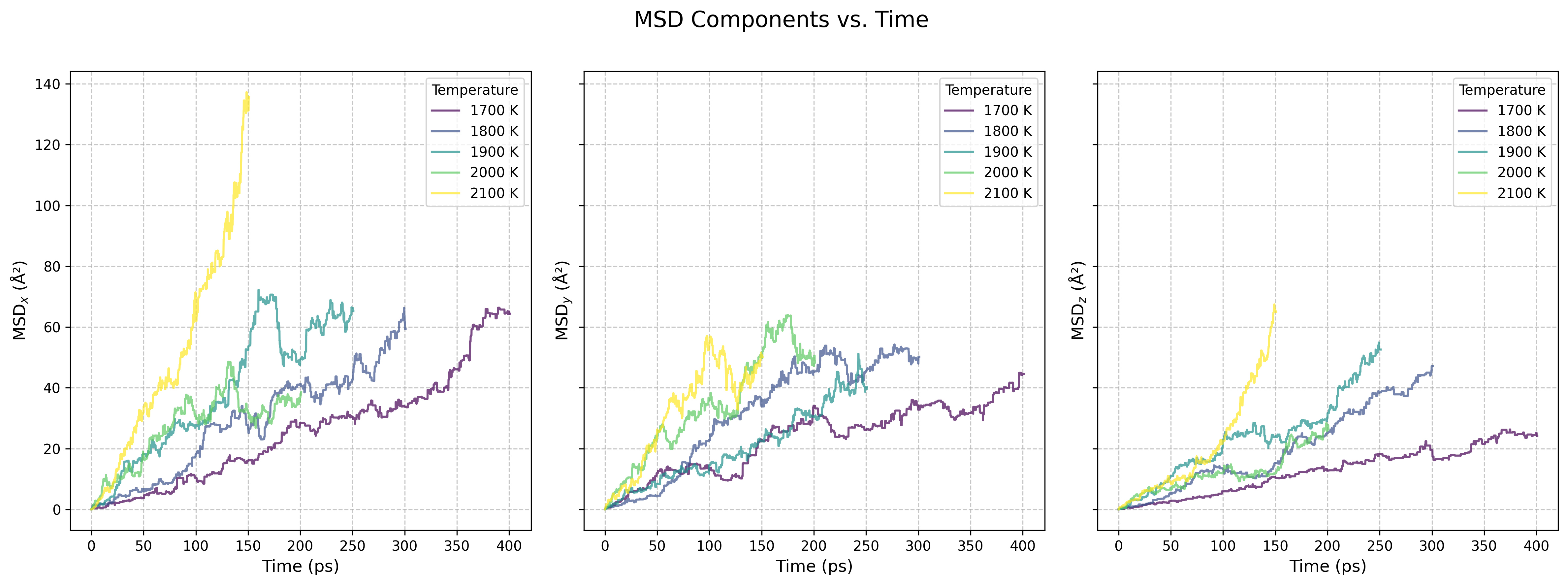
Note

This component-wise analysis requires significantly more sampling of hopping events than calculating the isotropic vacancy diffusivity. As seen in the example plots, insufficient sampling can lead to poor linearity in the MSD and reduced R² values for the Arrhenius fits.