Identifying Phase Transition

To follow this tutorial, please download and unzip Example5/ from this link (309 MB).

How to Identify Phase Transition

The core analyses in VacHopPy operate on a fixed set of lattice sites derived from your PATH_STRUCTURE file. Therefore, the results are reliable only when the system’s crystal structure remains stable throughout the MD simulation, without undergoing any phase transitions.

To help you verify this structural stability, VacHopPy provides the distance command. This command quantifies structural changes over time by comparing the MD trajectory against a reference structure. The theoretical background for this method is described in this paper.

The basic syntax for the distance command is:

vachoppy distance [PATH_TRAJ] [t_interval] [REFERENCE_STRUCTURE]

Command Arguments

PATH_TRAJ

Paths to the full set of HDF5 trajectory files for all species in the system (e.g., TRAJ_Ti.h5 TRAJ_O.h5 for TiO2 system).
t_interval

A time interval (in ps) used to average atomic positions. This coarse-graining reduces the impact of thermal fluctuations. A small value between 0.05–0.1 ps is generally sufficient, as this analysis aims to capture the overall trend and is therefore not highly sensitive to the specific t_interval value.
REFERENCE_STRUCTURE

Path to the reference structure file for comparison. Supports any format compatible with Atomic Simulatoin Environment (ASE).

Understanding Fingerprints and Optional Flags

The distance command works by converting each atomic structure into a fingerprint vector. This vector uniquely represents the structure, and the command calculates the difference between the fingerprint of the reference structure and the fingerprint at each MD time step.

Accurate results depend on well-calculated fingerprints, which can be tuned with the following flags:

--Rmax: Cutoff radius (Å) for the fingerprint. (default: 10.0)
--delta: Discretization step (Å). (default: 0.08)
--sigma: Gaussian broadening (Å) for the fingerprint. (default: 0.03)

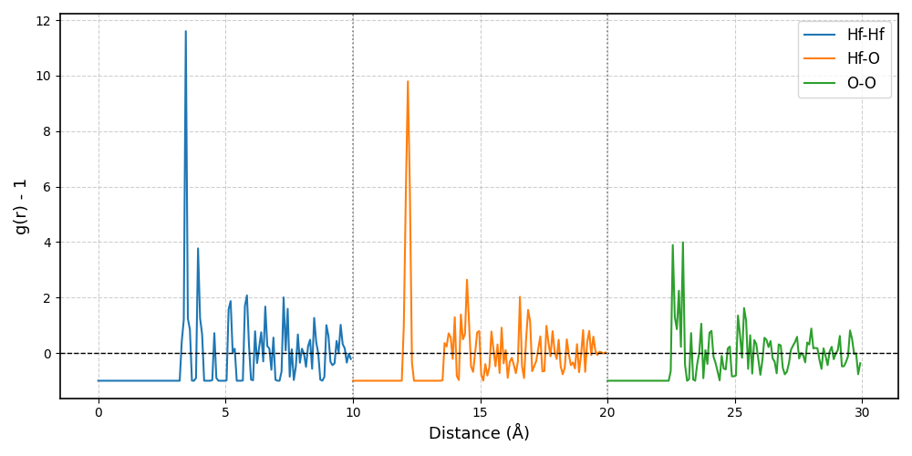
In most cases, the default values provide reliable results. To ensure your parameters are appropriate, you can visualize the fingerprint of your REFERENCE_STRUCTURE using the fingerprint command:

vachoppy fingerprint [PATH_STRUCTURE]

A well-generated fingerprint should converge to -1 at r=0 and approach 0 as r → ∞. An example is shown below:

Running the Analysis

Navigate into the Example5/ directory you downloaded. In this directory, you will find four HDF5 files and two structure files:

cd path/to/Example5/
ls
# >> TRAJ_Hf_2200K.h5  TRAJ_O_2200K.h5  TRAJ_Hf_1600K.h5  TRAJ_O_1600K.h5  
# >> POSCAR_MONOCLINIC  POSCAR_TETRAGONAL 

TRAJ_..._1600K.h5 and TRAJ_..._2200K.h5

These are two sets of HDF5 files for a monoclinic HfO₂ supercell containing one oxygen vacancy, simulated at 1600 K and 2200 K, respectively.
POSCAR_MONOCLINIC and POSCAR_TETRAGONAL

These are the reference structure files for the perfect, vacancy-free monoclinic and tetragonal phases of HfO₂.

Case 1: High-Temperature Simulation (2200 K)

Let’s first analyze the 2200 K simulation, which is above the known experimental transition temperature for HfO₂. We will measure the structural distance relative to both the initial monoclinic phase and the potential final tetragonal phase.

1. Compare against the Monoclinic structure:

Execute the following command:

vachoppy distance TRAJ_*_2200K.h5 0.05 POSCAR_MONOCLINIC

This command produces the following plot:

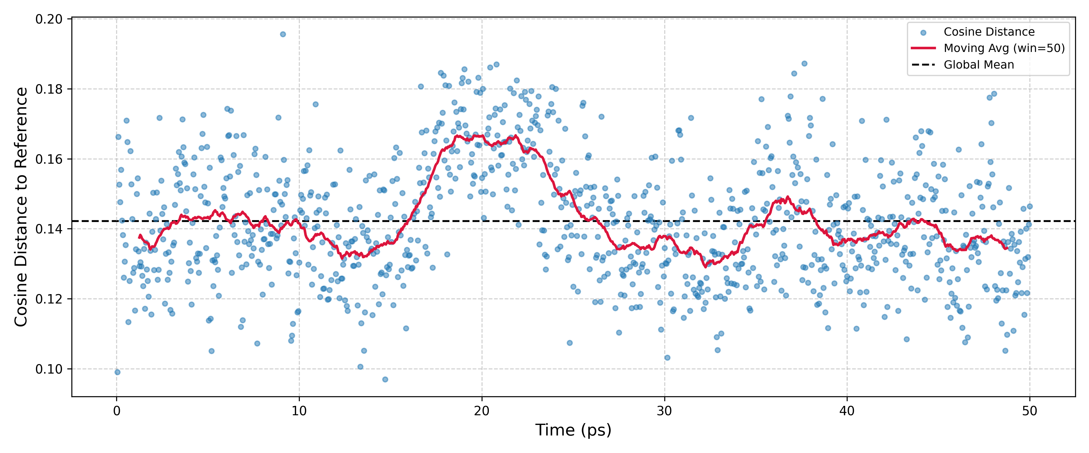
The red line, representing the average structural distance, shows a distinct drift away from the monoclinic reference structure around the 20 ps. For this analysis, the absolute y-values are not meaningful, and the important feature is the relative change. By default, the output files will be saved in the fingerprint_trace/ directory.

Compare against the Tetragonal structure:

Execute the following command:

vachoppy distance TRAJ_*_2200K.h5 0.05 POSCAR_TETRAGONAL

This command yields a contrasting result:

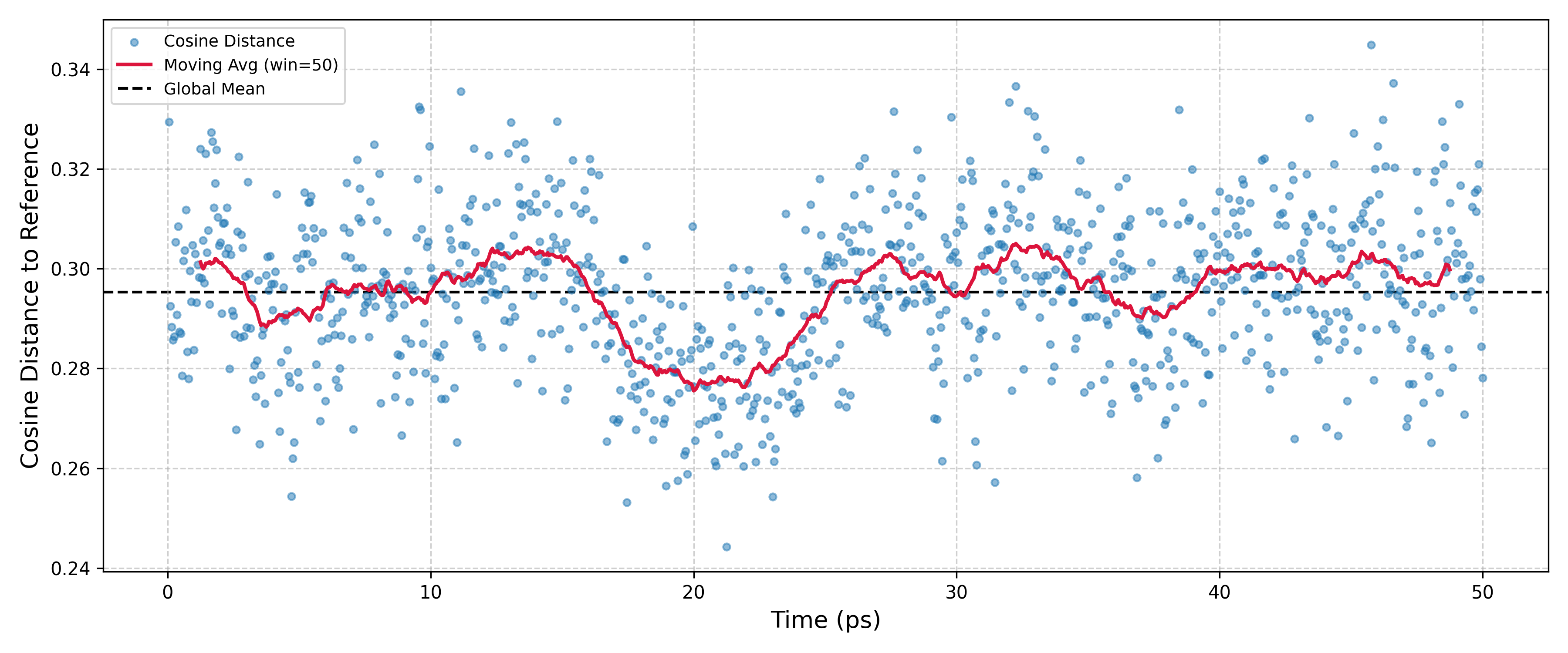
Here, the structure moves closer to the tetragonal reference at the same 20 ps mark. Together, these plots strongly suggest that a phase transition is occurring.

Note

It is important to remember that this simulation was run in an NVT ensemble, meaning the simulation cell’s lattice parameters are fixed to the monoclinic phase. Despite this constraint, the local atomic arrangement clearly trends towards a tetragonal configuration after 20 ps. This indicates an incipient phase transition.

Indeed, if a structural snapshot from around the 20 ps is relaxed, it converges to the tetragonal HfO₂ structure. (Structural snapshots can be obtained using the vachoppy.utils.Snapshot module.)

Case 2: Low-Temperature Comparison (1600 K)

For comparison, let’s run the same analysis on the 1600 K simulation, which is below the known transition temperature.

Execute the following two commands:

vachoppy distance TRAJ_*_1600K.h5 0.05 POSCAR_MONOCLINIC
vachoppy distance TRAJ_*_1600K.h5 0.05 POSCAR_TETRAGONAL

The two commands produce the following plots, respectively:

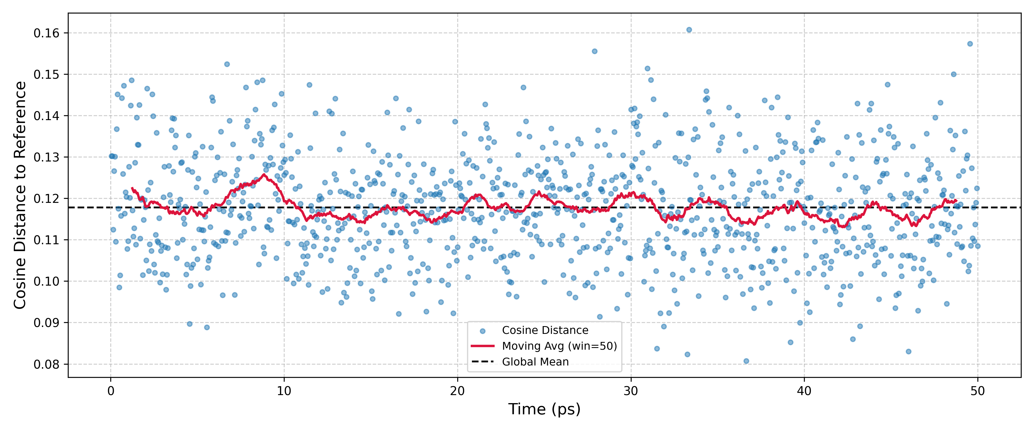
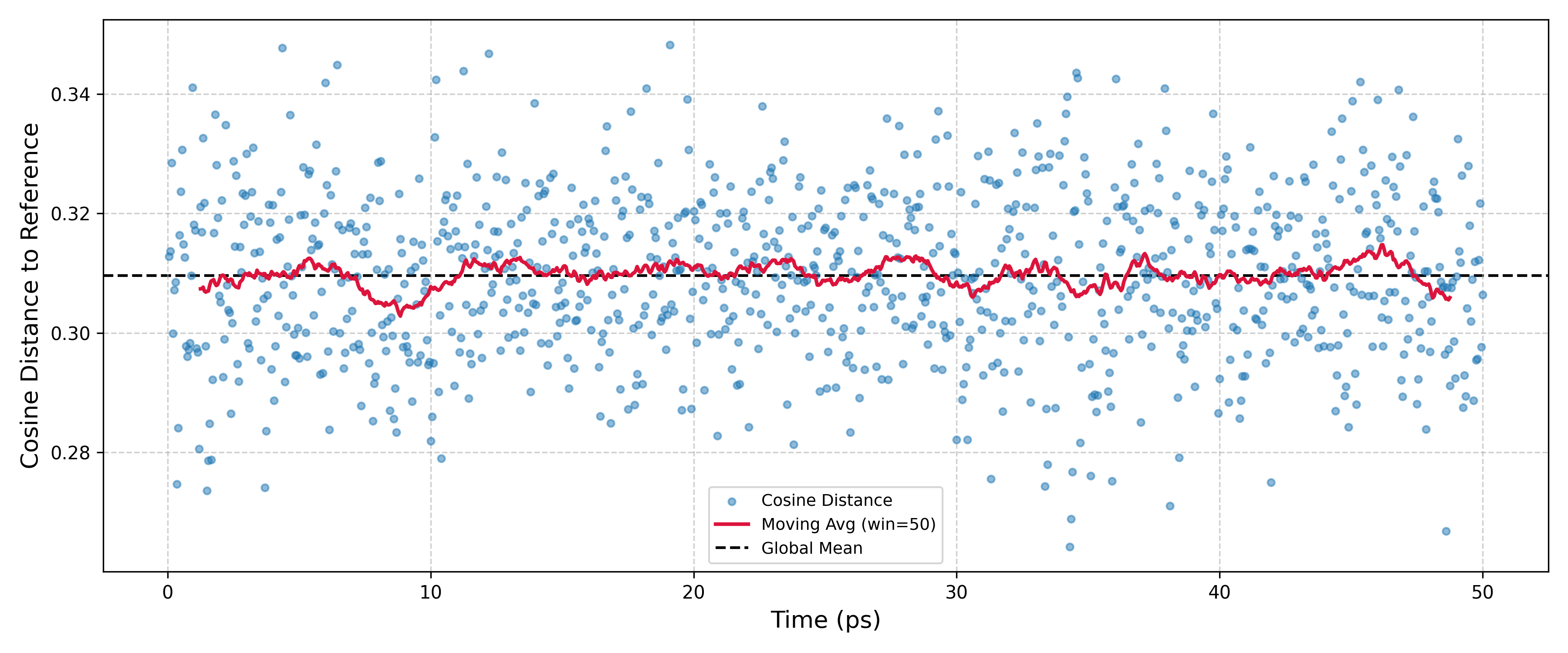
Unlike the 2200 K results, these plots show that the structure remains stable and close to the initial monoclinic phase throughout the simulation, with no significant drift towards the tetragonal phase. By comparing the two temperature cases, the distance command has successfully identified the onset of a phase transition at 2200 K.